Path-Space Differentiable Rendering: Supplemental Materials
Cheng Zhang1, Bailey Miller2, Kai Yan1, Ioannis Gkioulekas2, and Shuang Zhao1
1University of California, Irvine
2Carnegie Mellon University
1. Validation and Evaluation
1.1. Validation
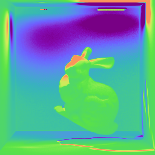
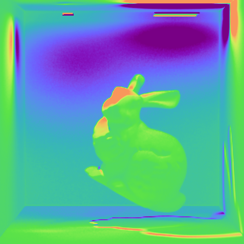
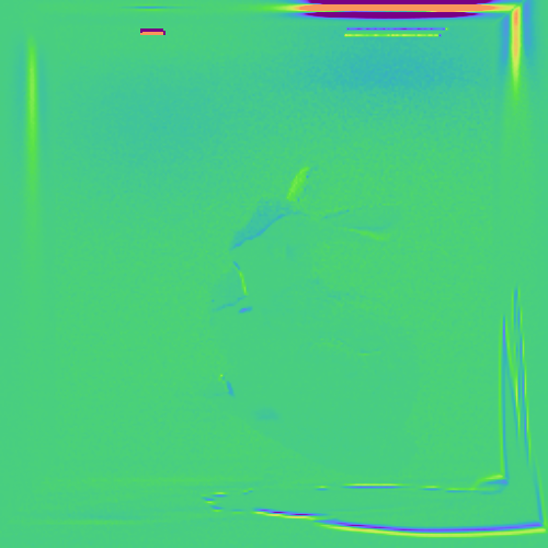
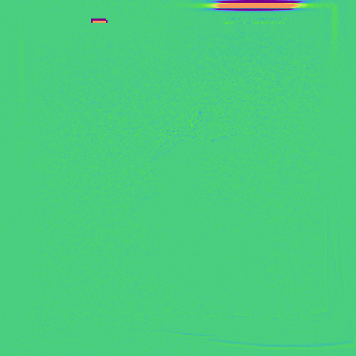
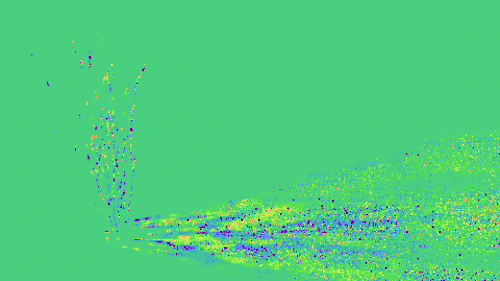
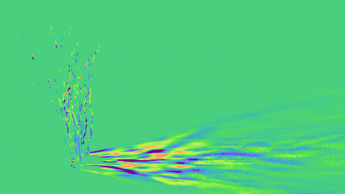
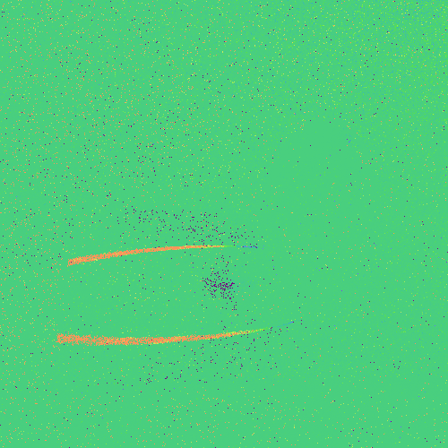
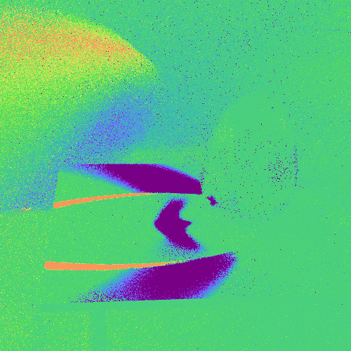
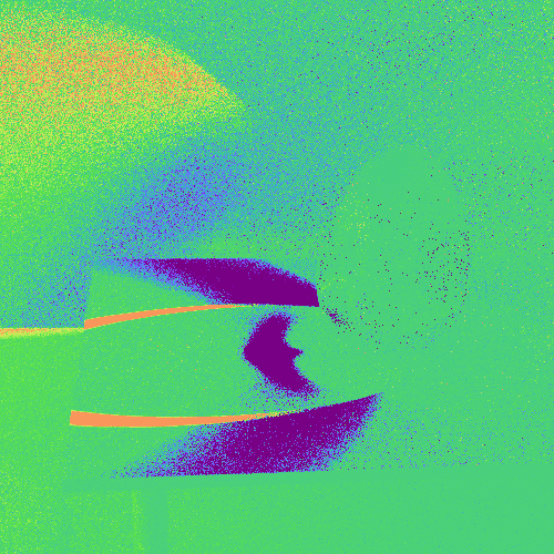
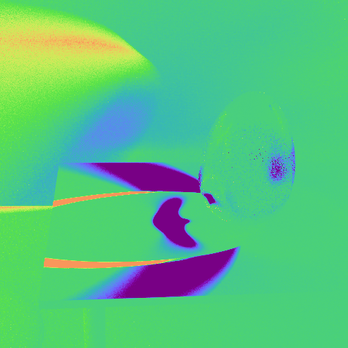
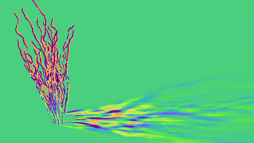
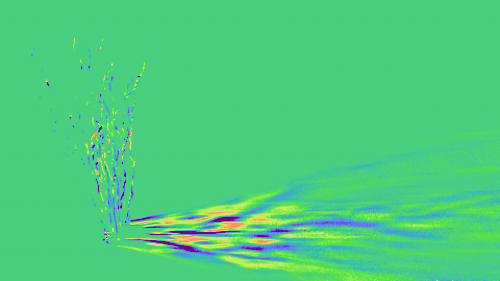
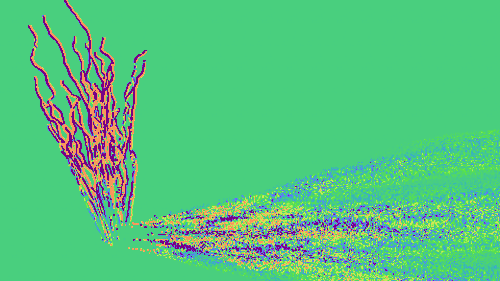
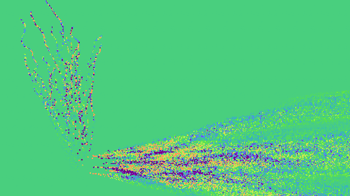
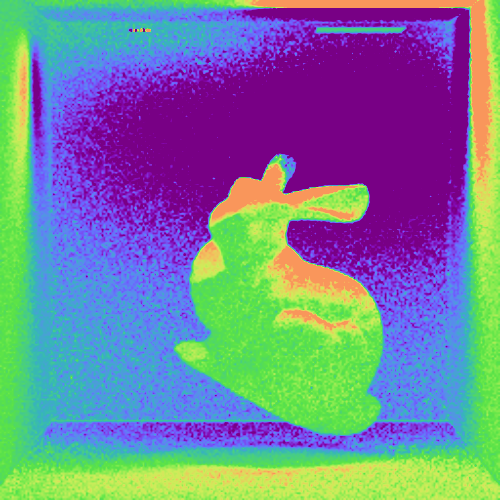
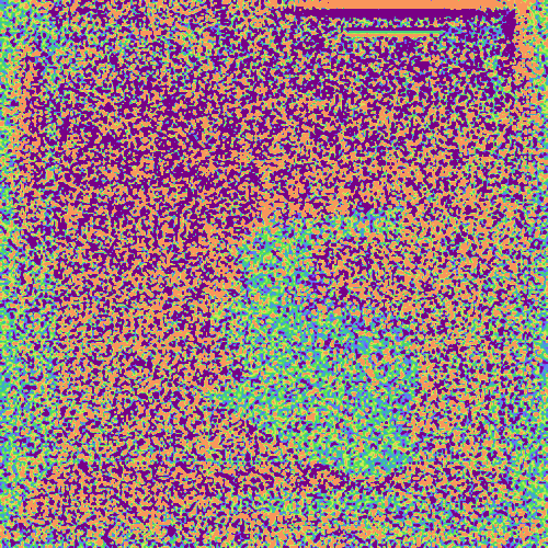
We validate our estimated derivatives by comparing to results computed using the finite-difference (FD) method in the following.
The derivatives and absolute differences are visualized using the color map below, and all visualizations in each row share the same color-map limits. The differences between the FD results and ours are due to FD bias and Monte Carlo noise.

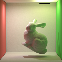
| Orig image |
Our deriv. |
FD (large spacing) |
Abs. diff |
 |
 |
 |
 |
|
|
FD (small spacing) |
Abs. diff |
|
|
 |
 |
| Orig image |
Our deriv. |
FD (large spacing) |
Abs. diff |
FD (small spacing) |
Abs. diff |
 |
 |
 |
 |
 |
 |
 |
 |
 |
 |
 |
 |
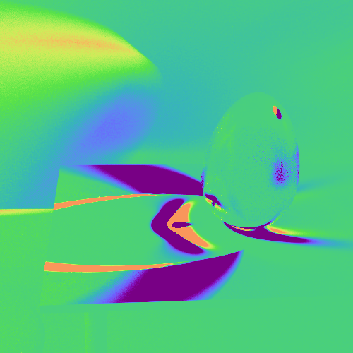
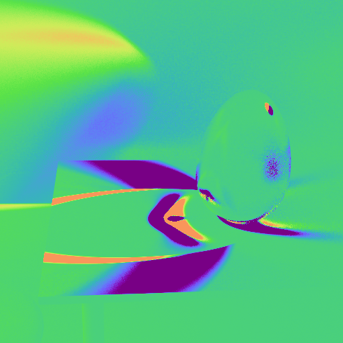
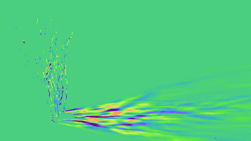
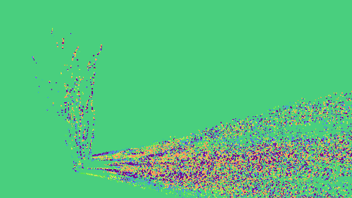
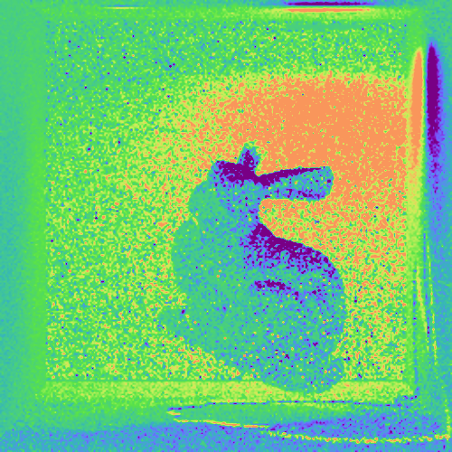
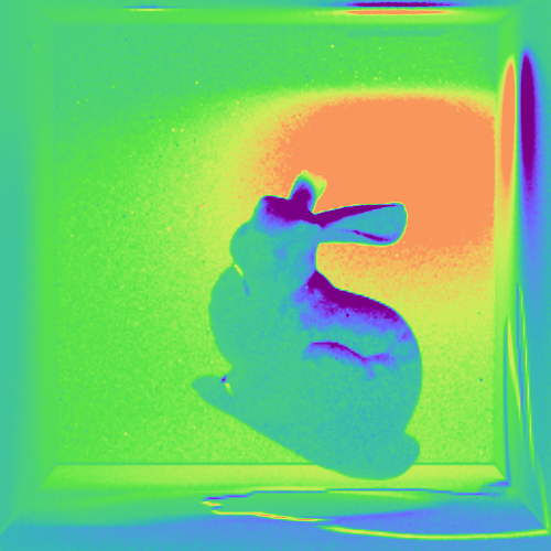
1.2. Per-Component Derivative Images
In what follows, we provide per-component visualizations for a few gradient images.
| All |
Main |
Boundary |
Primary Boundary |
|
 |
 |
 |
|
 |
 |
 |
|
 |
 |
 |
With next-event estimation (NEE) and importance sampling (IS) introduced in Section 6 of the paper, the efficiency of Monte-Carlo estimation of the boundary integral can be improved significantly.
We show equal-time comparisons of the boundary term estimated using different configurations below.
| Boundary |
Boundary (IS) |
Boundary (NEE) |
Boundary (NEE + IS) |
 |
 |
 |
 |
 |
 |
 |
 |
 |
 |
 |
 |
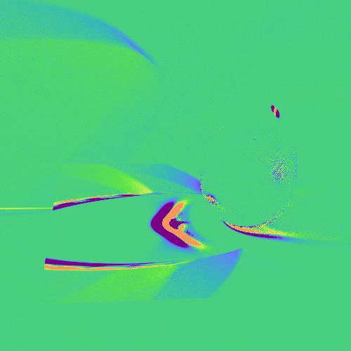
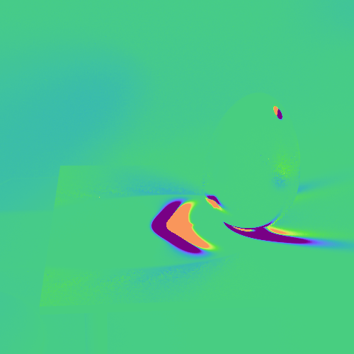
1.3. Derivative Image Comparisons
We demonstrate the effectiveness of our material differential path integral formulation by providing two equal-time comparisons of per-component gradient images between our technique and a state-of-the-art method DTRT [Zhang et al. 2019], which is largely equivalent (for the surface-only case) to Redner [Li et al. 2018].
|
All |
Main |
Boundary |
Primary |
| Our Method |
 |
 |
 |
 |
| DTRT |
 |
 |
 |
 |
| Our Method |
 |
 |
 |
 |
| DTRT |
 |
 |
 |
 |
2. Gradient-Based Inverse Rendering
We show inverse rendering examples using gradients estimated with our approach as well as a few state-of-the-art techniques.
The parameter RMSE plots show root-mean-square error of the optimized parameters. This information is not used by the optimizations.
The table below summarizes the performance statistics and optimization configurations for the inverse rendering examples.
The reported Time is measured per iteration on a workstation with 8-core intel i7-7820X CPU and Titan RTX graphics card.
| Scene |
# Param. |
# Iter. |
Time (Ours) |
Time (Reparam.) |
Time (DTRT) |
Time (Redner) |
Guiding Resol. |
| Branches |
1 |
140 |
0.5 s |
0.3 s |
5.66 s |
5.58 s |
40000 x 1 x1 |
| Puffer ball |
1 |
160 |
4.5 s |
1.5 s |
28.55 s |
|
100000 x 1 x 1 |
| Veach egg |
3 |
200 |
19.70 s |
153 s |
101.33 s |
|
5000 x 5 x 5 |
| Mug |
3 |
180 |
29.81 s |
|
|
|
N/A |
| Ring |
100 |
160 |
69.25 s |
|
|
|
N/A |
Inverse Rendering Comparison
 Left click the images below to start/pause; right click to reset the animations.
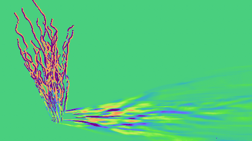
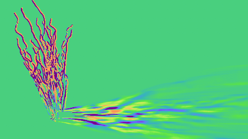
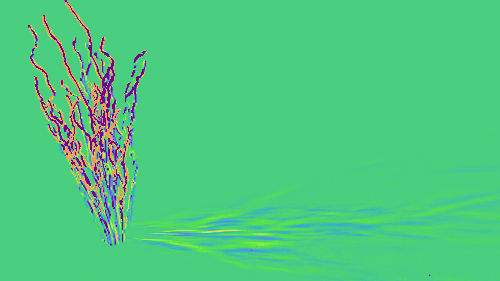
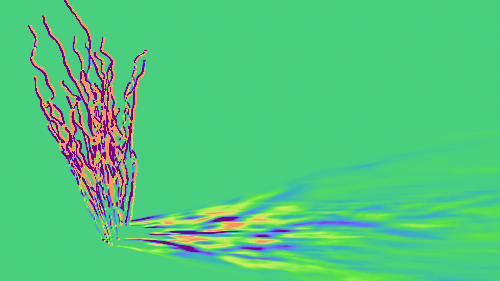
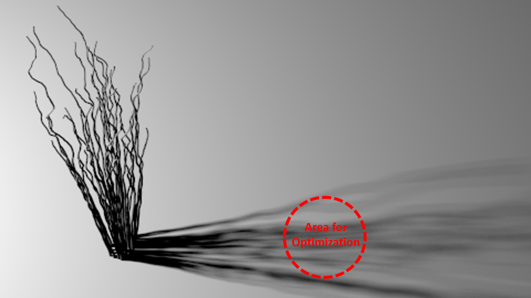
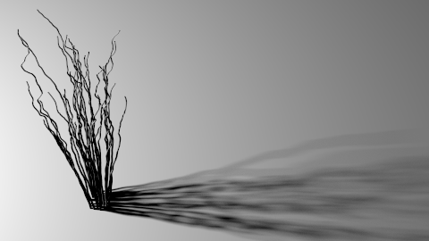
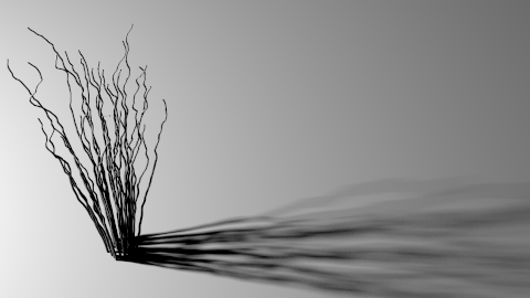
Branches
- This example contains a few twisted pipes lit by a small area source and is rendered with direct illumination only.
- We search for the rotation angle of the tree (around the vertical axis) by looking at its shadow.
-
All comparisons are equal-sample.
| Initial state |
Final state |
 |
 |
Target rotation = 0.2 radian:
| Initial state |
Final state |
 |
 |
Target rotation = 0.6 radian:
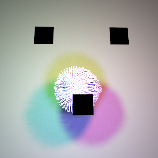
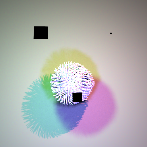
Puffer ball
- This example contains a highly-detailed pufferball mesh with over one million faces illuminated by four area lights of red, green and blue colors, creating the colored shadows on the ground.
- For each light, we use a single parameter to control its size and intensity such that the total power remains constant.
-
All comparisons are equal-sample.
| Initial state |
Final state |
 |
 |
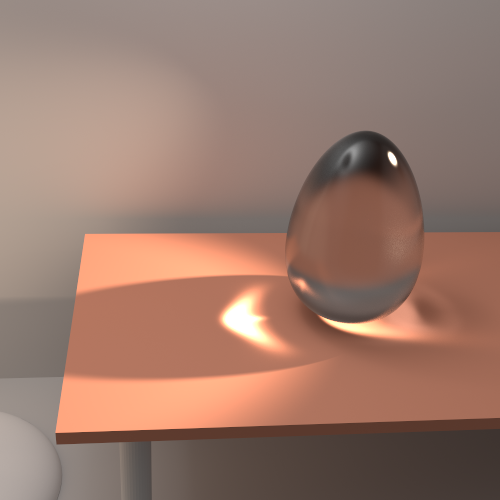
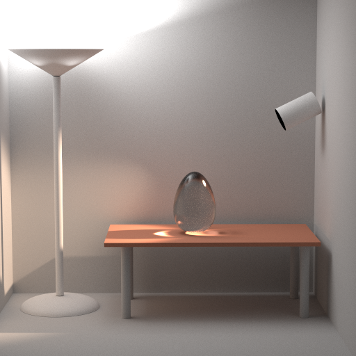
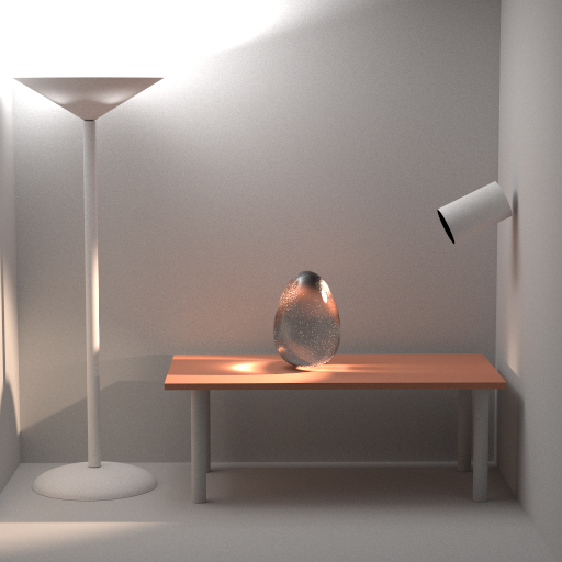
Veach Egg
- Modeled after a scene created by Eric Veach.
- We search for (i) the refractive index of the glass egg, and (ii) the position of emitter attached to the side wall.
- All comparisons equal-time.
| Initial state |
Final state |
 |
 |
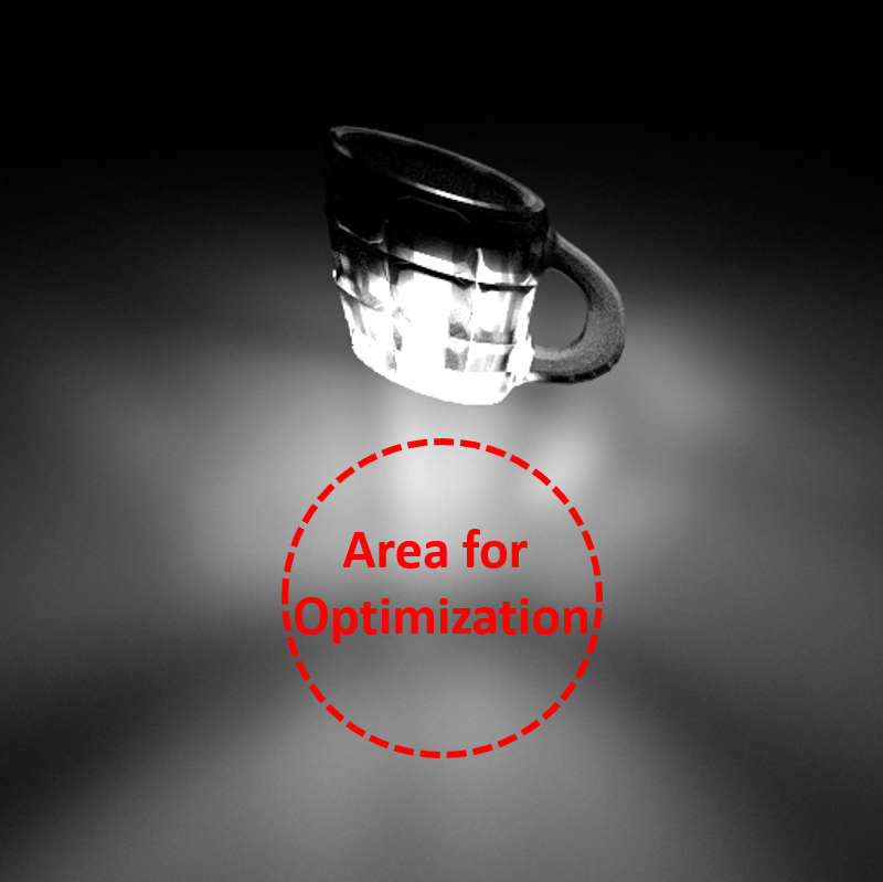
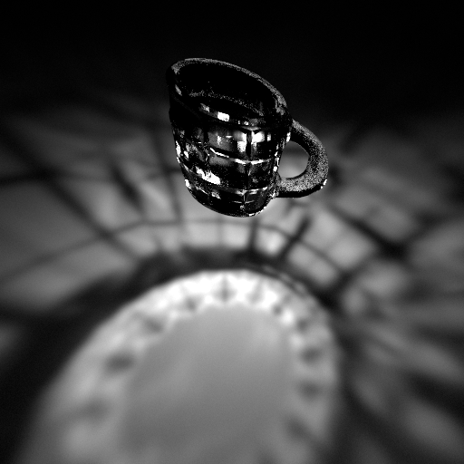
Glass Mug
- This example contains a glass mug with a small area light inside.
- We search for (i) the rotation of the glass mug (along a fixed axis), (ii) the vertical placement of the emitter, and (iii) the roughness of the glass mug.
- All comparisons are equal-time.
| Initial state |
Final state |
 |
 |
Generic Inverse Rendering
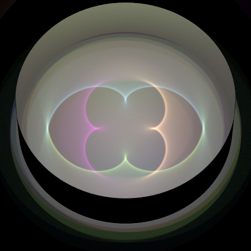
Ring Caustics
- This example contains a silver ring illuminated by four area lights with different colors.
- We optimize the cross-sectional shape of this ring parameterized using 100 variables.
| Initial state |
Final state |
 |
 |