A Differential Theory of Radiative Transfer:
Supplemental Materials

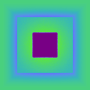
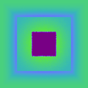
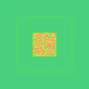
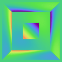
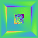
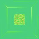
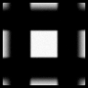
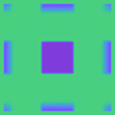
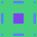
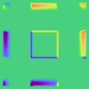
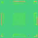
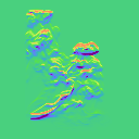
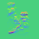
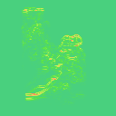
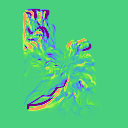
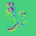
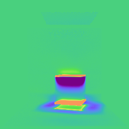
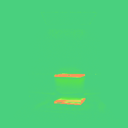
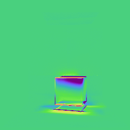
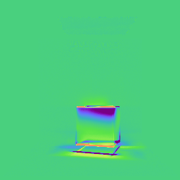
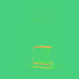
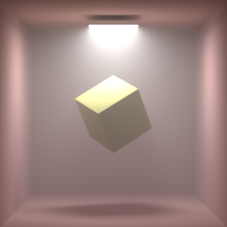
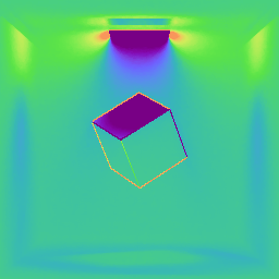
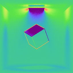
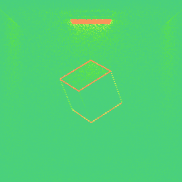
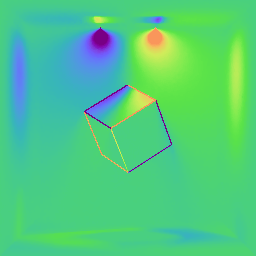
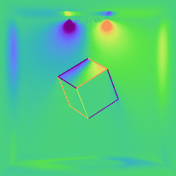
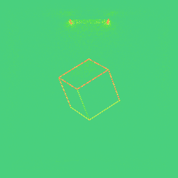
We validate our estimated derivatives by comparing to finite-difference (FD) results. The derivatives and absolute differences are visualized using the following colormap:

All visualizations in each row share the same color-map limits. The differences between the FD results and ours are due to FD bias and Monte Carlo noise.

Orig image	Ours 1	FD 1	Abs. diff	Ours 2	FD 2	Abs. diff

Here we show inverse rendering examples using gradients estimated with our approach.

The images under different viewing configurations (indicated with "diff. view") are not used for gradient-based optimization but to visualize the iterative refinement of scene parameters driven by the optimization.

• The opt. loss plots illustrate the change of our image-based loss function whose gradients drive the optimizations.
• The parameter diff. plots show the difference between the optimized parameters and the references. This information is not used by the optimizations.

The table below summarizes the performance statistics and optimization configurations for the inverse rendering examples. Time is measured in CPU core minutes per iteration.

Scene	# Param.	# Iter.	Time
Disco Ball	2	110	22
Glass 1	4	80	12.2
Camera pose	3	220	9.3
Glossy Reflector	9	200	23.6
Shape blending 1	1	100	3.0
Shape blending 2	1	50	6.4
Shadow 1	3	100	9
Shadow 2	2	60	7.6
Multilayer	3	50	31
Spotlight 1	12	200	11.2
Spotlight 2	12	110	11.2
Logo	101	100	27.2
Point light source	3	150	0.16
High-order geometry	3	150	13.2
Smooth dielectric IOR	1	50	0.96

Disco Ball

• This example contains a dodecahedron emitter within a homogeneous medium.
• We search for the orientation of the emitter.

Glass 1

• This example involves an apple embedded in a cube with light-absorbing medium and rough dielectric interface.
• We search for (i) the spatial location of the apple (ii) the surface roughness of the cube.

Camera pose

• This example contains a heterogeneous medium lit by an area light.
• We search for the spatial location and tilt angle of the camera.

Glossy reflector

• This example contains a glossy reflector and heterogeneous medium.
• We search for the spatial locations of the reflector's vertices to match the reflection of the medium.

Spotlight 1

• This example contains a glossy teapot within a homogeneous medium lit by two small spotlights.
• We search for the orientations and the emission colors of the spotlights.

Shape blending 1

• This example contains an area light source whose shape is given by a linear blending of two different polygons.
• We search for the blending weight with the light outside the field of view.

Shape blending 2

• This example contains randomly placed and oriented grains whose shapes are given by a linear blending of two different polyhedra.
• We search for the blending weight using a distant view where individual grains are barely visible.

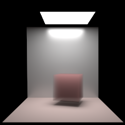
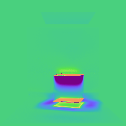
Shadow 1

• This example has a Cornell-box-like configuration with a homogeneous translucent cube and a glossy back wall.
• We search for the spatial location of the translucent cube by only looking at its shadow.

Shadow 2

• This example contains a heterogeneous participating medium lit by a small area source.
• We search for (i) the orientation and (ii) the optical density of a heterogeneous medium by only looking at its shadow.

Multilayer

• This example involves a two-layer medium that has scattering parameters analogous to human skin and a dark object embedded within.
• We search for the spatial location of the embedded object.

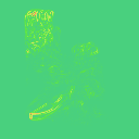
Spotlight 2

• This example contains a glossy teapot within a homogeneous medium lit by two small spotlights.
• We search for the orientations and the colors of the spotlights using a hand-drawn image as input.

Logo

• This example contains a granular material with translucent grains with spatially varying colors and sizes.
• Given an input image, we search for the colors and sizes of the grain clusters from a distant view where individual grains are barely visible.

We now show proof-of-concept examples generated with generalized versions of our derivation from the supplemental document.

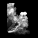
All the result images are grayscale with pixel intensities encoded in false colors using the following color map:

Point light source

• This example involves a point light source and a triangle occluder contained in an infinite homogeneous medium.
• We search for the spatial location of the light source by only looking at the volumetric shadow casted by the triangle.

High-order geometry

• This example involves a sphere lit by an area source in an infinite homogeneous medium.
• We search for the spatial location of the sphere.

Smooth dielectric IOR

• This example involves a semi-infinite heterogeneous medium with a smooth dielectric interface.
• We search for the refractive index (IOR) of the medium.