CS114 Project 2:
Monte Carlo Integration & Path Tracing
Due: Wednesday May 6, 2020 (23:59 Pacific Time)
Part 1. Monte Carlo Integration
In this part, you will implement several Monte Carlo estimators for computing integrals and compare their efficiencies.
Please submit a ZIP package for this task containing:
- A report (in PDF format) with all experimental results (see individual tasks for details);
- All your source code. You can use any programming language, but C++ is highly recommended as your C++ implementations will come in handy for Part 2.
Task 1. One-Dimensional Problems
Task 1-1. Warming up
Compute the following integral $$ I = \int_{-2}^2 \exp\left(-\frac{x^2}{2}\right)\,\mathrm{d}x, $$ (where $\exp()$ denotes the natural exponential function) using Monte Carlo integration with density function $$ p(x) \equiv \frac{1}{4} \quad\text{for all $-2 \leq x < 2$.} $$
You should start with drawing $N = 100\ 000$ samples $x_1,\ x_2,\ \ldots,\ x_N \in [-2, 2)$:
- If you choose to implemenmt this task with C++ (which is recommended!), use C++11's pseudo-random number generator instead of the outdated rand() function.
- For Python users, use numpy's random module.
- For Java users, use the built-in Random class.
With $x_1,\ x_2,\ \ldots,\ x_N$ generated, you then need to evaluate $\hat{I}_{\!1},\ \hat{I}_{\!2},\ \ldots,\ \hat{I}_{\!N}$ given by: $$ \hat{I}_{\!j} = \frac{\exp(-x_j^2/2)}{p(x_j)} \quad\text{for $j = 1,\ 2,\ \ldots, N$}, $$ and include the following in your report:
- Sample mean: $$ \bar{I} := \frac{1}{N} \sum_{j = 1}^N \hat{I}_{\!j}, $$
- (Scaled) deviation: $$ \bar{s} = \frac{2s}{\sqrt{N}}, $$ with $s$ being sample standard deviation given by $$ s := \sqrt{\frac{\displaystyle\sum_{j=1}^N \left(\hat{I}_{\!j} - \bar{I}\right)^2}{N - 1}}. $$ (See this if you are interested to know why $s$ has $N - 1$ instead of $N$ in its denominator.)
Please execute your code 10 times (with non-fixed random seeds), and you should get 10 sets of slightly different $\bar{I}$ and $\bar{s}$ values. Report all of them (rounded to three decimal places) in a table that looks like:
| Round | $\bar{I}$ | $\bar{s}$ |
| 1 | x.xxx | x.xxx |
| 2 | x.xxx | x.xxx |
| $\vdots$ | $\vdots$ | $\vdots$ |
| 10 | x.xxx | x.xxx |
Remark: If you implement everything correctly, the interval $[ \bar{I} - \bar{s},\ \bar{I} + \bar{s} ]$ should contain the correct answer 2.3926 about 95% of the time. As a result, this interval is called a 95% confidence interval.
Task 1-2. Integrals over Unbounded Intervals
Compute the following integral $$ I = \int_{1}^{\infty} \exp\left(-\frac{x^2}{2}\right)\,\mathrm{d}x. $$
Since this integral is defined over the unbounded interval $[1, \infty)$, uniform distributions cannot be used. Instead, please draw $\xi$ uniformly from $[0, 1)$, and set $$ x = 1 - \frac{\log \xi}{\lambda} $$ (where $\log()$ is the natural logarithm function) with some fixed $\lambda > 0$. In this case, $x$ will be distributed exponentially with probability density $$ p(x ; \lambda) = \lambda \exp(-\lambda (x - 1)). $$
Please try three different $\lambda$ values: 0.1, 1.0, and 10.0. For each $\lambda$, create a table with 10 sets of $\bar{I}$ and $\bar{s}$ values each of which uses $N = 100\ 000$ independent samples (similar to Task 1-1). Then, discuss in your report:
- Which $\lambda$ value has led to an estimator with best efficiency?
- Optional: Why? (You do not have to provide rigorous math, but try including some high-level explanations.)
Task 2. Integrals over Unit Spheres
Task 2-1. Surface Area of the Hemisphere
As discussed in class, the surface area of a unit hemisphere can be computed using sphere coordinates ($\theta$, $\phi$) as $$ \int_0^{2\pi} \int_0^{\pi/2} \sin\theta \mathrm{d}\theta \mathrm{d}\phi. $$ Let $A := [0, \frac{\pi}{2}) \times [0, 2\pi)$ be a 2D rectangle, then the previous integral can be rewritten as $$ I := \int_A \sin({\bf x}[1])\,\mathrm{d}{\bf x}, $$ where ${\bf x}$ is a 2D vector and ${\bf x}[1]$ denotes its first component (that is, if ${\bf x} = (a, b)$, then ${\bf x}[1] = a$).
Use Monte Carlo integration to estimate $I$ by uniformly sampling ${\bf x}$ from $A$. That is, generating each sample by:
- Setting $$ {\bf x}_j \gets \left(\frac{\pi}{2} \xi_{j,1},\ 2\pi \xi_{j,2} \right) \quad\text{for $j = 1, 2, \ldots, N$,} $$ with $\xi_{j,1}$ and $\xi_{j,2}$ drawn independently from $U[0, 1)$;
- Evaluating $\hat{I}_{\!j}$ accordingly.
Include a table similar to Task 1-1 in your report.
Task 2-2. Arbitrary Spherical Function
Let $$ \begin{aligned} \theta &= \arccos(\xi_1),\\ \phi &= 2\pi\xi_2, \end{aligned} $$ where $\xi_1,\ \xi_2$ are drawn independently from $U[0, 1)$. Then it can be shown that $\omega := (\theta, \phi)$ in spherical coordinates is distributed uniformly over the hemisphere centered at (0, 0, 0). That is, $$ p(\omega) \equiv \frac{1}{2\pi}, $$ for all $\omega$'s generated this way.
Use this sampling scheme to estimate the following integral: $$ I = \int_{\Omega_+} (\cos\theta\,\sin\theta\,\cos\phi)^2\,\mathrm{d}\omega, $$ where $\Omega_+$ denotes the entire unit hemisphere with $\theta \in [0, \frac{\pi}{2})$. Include a table similar to Task 1-1 in your report.
Task 3. Estimating Radiant Flux
Consider a simple 3D scene with two objects:
- A unit square $R$ in the XOY plane centered at the origin (i.e., with two corners at $(-0.5, -0.5, 0)$ and $(0.5, 0.5, 0)$);
- A spherical light source $S$ centered at $(1, 1, 5)$ with radius 1.
This light source is a uniform emitter: its emitted radiance (at any point on the surface in any direction) is fixed to $L = 100$.
Then, the radiant flux (i.e., power) received by $R$ equals
$$
P = \int_R \int_{\Omega_+} L \cdot \chi({\bf x}, \omega) \cdot \cos\theta\,\mathrm{d}{\omega}\,\mathrm{d}{\bf x},
$$
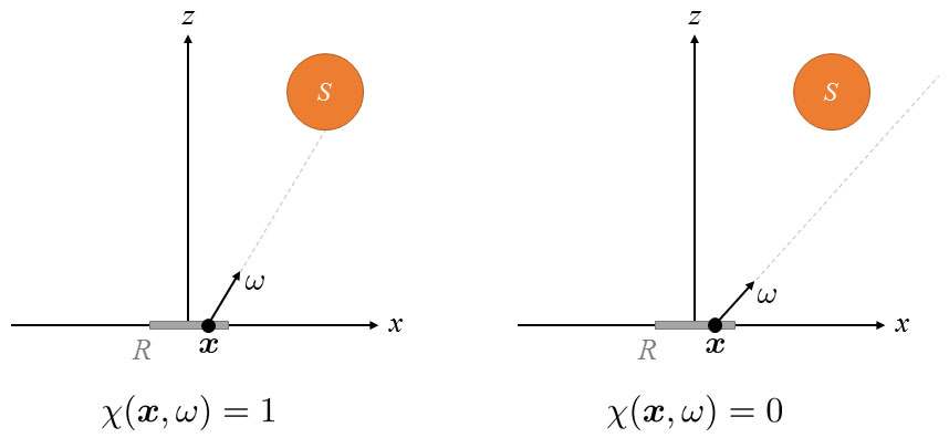
where $\theta$ is the angle between $\omega$ and the Z-axis, and $\chi$ is an indicator function given by
$$
\chi({\bf x}, \omega) = \begin{cases}
1 & \text{if ray $({\bf x}, \omega)$ hits $S$,}\\
0 & \text{otherwise}.
\end{cases}
$$
Two examples are shown below:
Use Monte Carlo integration to estimate $P$ by uniformly sampling ${\bf x} \in R$ and $\omega \in \Omega_+$. Pick proper number of samples so that the resulting estimation is accurate to one decimal place. Report your estimated $P$ value and the number of samples used.
Extra Credit: Use non-uniform sampling for $\omega$ to achieve better convergence rate. Describe in your report:
- The density function you picked;
- The way you generate samples of $\omega$;
- The number of samples needed to achieve the same accuracy (of one decimal place).